 Active Topics
  Memberlist
  Calendar
  Search
  |
 Active Topics Active Topics  Memberlist Memberlist  Calendar Calendar  Search Search |
| |
| |
  |
| Author | Message | |||||||||||||||||||||||||||||||||||||||||||||||||||||||
|
sumana
Newbie 
Joined: 08Apr2007 Online Status: Offline Posts: 9 |
  Topic: Sorting Topic: SortingPosted: 08Apr2007 at 10:02pm |
|||||||||||||||||||||||||||||||||||||||||||||||||||||||
|
2.3 Sorting
One of the major applications in computer science
is the sorting of information in a table. Sorting algorithms arrange
items in a set according to a predefined ordering relation. The most
common types of data are string information and numerical information.
The ordering relation for numeric data simply involves arranging items
in sequence from smallest to largest and from largest to smallest,
which is called ascending and descending order respectively.
The
items in a set arranged in non-decreasing order are
{7,11,13,16,16,19,23}. The items in a set arranged in descending order
is of the form {23,19,16,16,13,11,7}
Similarly
for string information, {a, abacus, above, be, become, beyond}is in
ascending order and { beyond, become, be, above, abacus, a}is in
descending order.
There
are numerous methods available for sorting information. But, not even
one of them is best for all applications. Performance of the methods
depends on parameters like, size of the data set, degree of relative
order already present in the data etc.
2.3.1 Selection sort
The idea in selection sort is to find the smallest value and place
it in an order, then find the next smallest and place in the right
order. This process is continued till the entire table is sorted.
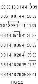
Consider the unsorted array,
a[1] a[2] a[8]
 2.3.2 Insertion sort
Insertion sort is a straight forward method that is useful for
small collection of data. The idea here is to obtain the complete
solution by inserting an element from the unordered part into the
partially ordered solution extending it by one element. Selecting an
element from the unordered list could be simple if the first element of
that list is selected.
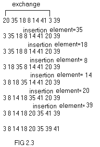
a[1] a[2] a[8]
 The changes undergone are shown in fig 2.3.
One
of the disadvantages of the insertion sort method is the amount of
movement of data. In the worst case, the number of moves is of the
order O(n2). For lengthy records it is quite time consuming.
2.3.3 Merge sort The changes undergone are shown in fig 2.3.
One
of the disadvantages of the insertion sort method is the amount of
movement of data. In the worst case, the number of moves is of the
order O(n2). For lengthy records it is quite time consuming.
2.3.3 Merge sort
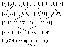
 Merge sort begins by interpreting the inputs as n sorted files
each of length one. These are merged pair wise to obtain n/2 files of
size two. If n is odd one file is of size one. These n/2 files are then
merged pair wise and so on until we are left with only one file. The
example in fig 2.4 illustrates the process of merge sort.
As
illustrated in the example merge sort consists of several passes over
the records being sorted. In the first pass files of size one are
merged. In the second pass the size of the files being merged is two.
In the ith pass the files being merged will be of size 2i-1. A total of log2n
passes are made over the data. Since, two files can be merged in linear
time, each pass of merge sort takes O(n) time. As there are log2n passes the total time complexity is O(n log2n). Merge sort begins by interpreting the inputs as n sorted files
each of length one. These are merged pair wise to obtain n/2 files of
size two. If n is odd one file is of size one. These n/2 files are then
merged pair wise and so on until we are left with only one file. The
example in fig 2.4 illustrates the process of merge sort.
As
illustrated in the example merge sort consists of several passes over
the records being sorted. In the first pass files of size one are
merged. In the second pass the size of the files being merged is two.
In the ith pass the files being merged will be of size 2i-1. A total of log2n
passes are made over the data. Since, two files can be merged in linear
time, each pass of merge sort takes O(n) time. As there are log2n passes the total time complexity is O(n log2n).for more details clik here: http://www.vyomworld.com/gate/cs/ada/2.3.asp Post Resume: Click here to Upload your Resume & Apply for Jobs |
||||||||||||||||||||||||||||||||||||||||||||||||||||||||
 IP Logged IP Logged |
||||||||||||||||||||||||||||||||||||||||||||||||||||||||
  |
||
Forum Jump |
You cannot post new topics in this forum You cannot reply to topics in this forum You cannot delete your posts in this forum You cannot edit your posts in this forum You cannot create polls in this forum You cannot vote in polls in this forum |
|
|

© Vyom Technosoft Pvt. Ltd. All Rights Reserved.