Active Topics
  Memberlist
  Calendar
  Search
 | Active Topics Memberlist Calendar Search |
|
| |
 Topic: Gate Study Material Graph theoretic algorithms Topic: Gate Study Material Graph theoretic algorithms |
  |
| Author | Message | |||||||||||||||||||||||||||||||||||||||||||||||||||||||||||||||||||||||||||||||||||||||||||||||||||||||||||||||||||||||||||||||||||||||||||||||||||||||||
|
Anamica
Newbie 
Joined: 04Apr2007 Online Status: Offline Posts: 9 |
  Topic: Gate Study Material Graph theoretic algorithms Topic: Gate Study Material Graph theoretic algorithmsPosted: 04Apr2007 at 10:41pm |
|||||||||||||||||||||||||||||||||||||||||||||||||||||||||||||||||||||||||||||||||||||||||||||||||||||||||||||||||||||||||||||||||||||||||||||||||||||||||
|
7.1 Single-source shortest path: Graphs can be used to represent the highway structure of a state or country with vertices representing cities and edges representing sections of highway. The edges can then be assigned weights which may be either the distance between the two cities connected by the edge or the average time to drive along that section of highway. A motorist wishing to drive from city A to B would be interested in answers to the following questions:
 The
problems defined by these questions are special case of the path
problem we study in this section. The length of a path is now defined
to be the sum of the weights of the edges on that path. The starting
vertex of the path is referred to as the source and the last vertex the
destination. The graphs are digraphs representing streets. Consider a
digraph G=(V,E), with the distance to be traveled as weights on the
edges. The problem is to determine the shortest path from v0 to all the
remaining vertices of G. It is assumed that all the weights associated
with the edges are positive. The shortest path between v0 and some
other node v is an ordering among a subset of the edges. Hence this
problem fits the ordering paradigm.
Example:
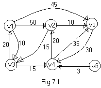
Consider the digraph of fig 7-1. Let the
numbers on the edges be the costs of travelling along that route. If a
person is interested travel from v1 to v2, then he encounters many
paths. Some of them are The
problems defined by these questions are special case of the path
problem we study in this section. The length of a path is now defined
to be the sum of the weights of the edges on that path. The starting
vertex of the path is referred to as the source and the last vertex the
destination. The graphs are digraphs representing streets. Consider a
digraph G=(V,E), with the distance to be traveled as weights on the
edges. The problem is to determine the shortest path from v0 to all the
remaining vertices of G. It is assumed that all the weights associated
with the edges are positive. The shortest path between v0 and some
other node v is an ordering among a subset of the edges. Hence this
problem fits the ordering paradigm.
Example:
Consider the digraph of fig 7-1. Let the
numbers on the edges be the costs of travelling along that route. If a
person is interested travel from v1 to v2, then he encounters many
paths. Some of them are
7.2 Minimum-Cost spanning trees Let G=(V,E) be an undirected connected graph. A sub-graph t = (V,E1) of G is a spanning tree of G if and only if t is a tree. Above figure shows the complete graph on four nodes together with three of its spanning tree.
Spanning trees have many applications.
For example, they can be used to obtain an independent set of circuit
equations for an electric network. First, a spanning tree for the
electric network is obtained. Let B be the set of network edges not in
the spanning tree. Adding an edge from B to the spanning tree creates a
cycle. Kirchoffs second law is used on each cycle to obtain a circuit
equation.
Another application of spanning trees
arises from the property that a spanning tree is a minimal sub-graph G
of G such that V(G) = V(G) and G is connected. A minimal sub-graph
with n vertices must have at least n-1 edges and all connected graphs
with n-1 edges are trees. If the nodes of G represent cities and the
edges represent possible communication links connecting two cities,
then the minimum number of links needed to connect the n cities is n-1.
the spanning trees of G represent all feasible choice.
In practical situations, the edges have
weights assigned to them. Thse weights may represent the cost of
construction, the length of the link, and so on. Given such a weighted
graph, one would then wish to select cities to have minimum total cost
or minimum total length. In either case the links selected have to form
a tree. If this is not so, then the selection of links contains a
cycle. Removal of any one of the links on this cycle results in a link
selection of less const connecting all cities. We are therefore
interested in finding a spanning tree of G. with minimum cost since the
identification of a minimum-cost spanning tree involves the selection
of a subset of the edges, this problem fits the subset paradigm.
7.2.1 Prims Algorithm
A greedy method to obtain a minimum-cost
spanning tree builds this tree edge by edge. The next edge to include
is chosen according to some optimization criterion. The simplest such
criterion is to choose an edge that results in a minimum increase in
the sum of the costs of the edges so far included. There are two
possible ways to interpret this criterion. In the first, the set of
edges so far selected form a tree. Thus, if A is the set of edges
selected so far, then A forms a tree. The next edge(u,v) to be included
in A is a minimum-cost edge not in A with the property that A U {(u,v)}
is also a tree. The corresponding algorithm is known as prims
algorithm.
For Prims algorithm draw n isolated
vertices and label them v1, v2, v3,
vn. Tabulate the given weights of
the edges of g in an n by n table. Set the non existent edges as very
large. Start from vertex v1 and connect it to its nearest neighbor
(i.e., to the vertex, which has the smallest entry in row1 of table)
say Vk. Now consider v1 and vk as one subgraph and connect this
subgraph to its closest neighbor. Let this new vertex be vi. Next
regard the tree with v1 vk and vi as one subgraph and continue the
process until all n vertices have been connected by n-1 edges.
Consider the graph shown in fig 7.3. There are 6 vertices and 12 edges. The weights are tabulated in table given below.
Above figure shows the complete graph on four nodes together with three of its spanning tree.
Spanning trees have many applications.
For example, they can be used to obtain an independent set of circuit
equations for an electric network. First, a spanning tree for the
electric network is obtained. Let B be the set of network edges not in
the spanning tree. Adding an edge from B to the spanning tree creates a
cycle. Kirchoffs second law is used on each cycle to obtain a circuit
equation.
Another application of spanning trees
arises from the property that a spanning tree is a minimal sub-graph G
of G such that V(G) = V(G) and G is connected. A minimal sub-graph
with n vertices must have at least n-1 edges and all connected graphs
with n-1 edges are trees. If the nodes of G represent cities and the
edges represent possible communication links connecting two cities,
then the minimum number of links needed to connect the n cities is n-1.
the spanning trees of G represent all feasible choice.
In practical situations, the edges have
weights assigned to them. Thse weights may represent the cost of
construction, the length of the link, and so on. Given such a weighted
graph, one would then wish to select cities to have minimum total cost
or minimum total length. In either case the links selected have to form
a tree. If this is not so, then the selection of links contains a
cycle. Removal of any one of the links on this cycle results in a link
selection of less const connecting all cities. We are therefore
interested in finding a spanning tree of G. with minimum cost since the
identification of a minimum-cost spanning tree involves the selection
of a subset of the edges, this problem fits the subset paradigm.
7.2.1 Prims Algorithm
A greedy method to obtain a minimum-cost
spanning tree builds this tree edge by edge. The next edge to include
is chosen according to some optimization criterion. The simplest such
criterion is to choose an edge that results in a minimum increase in
the sum of the costs of the edges so far included. There are two
possible ways to interpret this criterion. In the first, the set of
edges so far selected form a tree. Thus, if A is the set of edges
selected so far, then A forms a tree. The next edge(u,v) to be included
in A is a minimum-cost edge not in A with the property that A U {(u,v)}
is also a tree. The corresponding algorithm is known as prims
algorithm.
For Prims algorithm draw n isolated
vertices and label them v1, v2, v3,
vn. Tabulate the given weights of
the edges of g in an n by n table. Set the non existent edges as very
large. Start from vertex v1 and connect it to its nearest neighbor
(i.e., to the vertex, which has the smallest entry in row1 of table)
say Vk. Now consider v1 and vk as one subgraph and connect this
subgraph to its closest neighbor. Let this new vertex be vi. Next
regard the tree with v1 vk and vi as one subgraph and continue the
process until all n vertices have been connected by n-1 edges.
Consider the graph shown in fig 7.3. There are 6 vertices and 12 edges. The weights are tabulated in table given below.
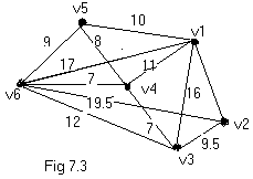
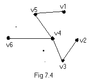
Start with v1 and pick the smallest entry in row1, which is either (v1,v2) or (v1,v5). Let us pick (v1, v5). The closest neighbor of the subgraph (v1,v5) is v4 as it is the smallest in the rows v1 and v5. The three remaining edges selected following the above procedure turn out to be (v4,v6) (v4,v3) and (v3, v2) in that sequence. The resulting shortest spanning tree is shown in fig 7.4. The weight of this tree is 41.5. 7.2.3 Kruskals Algorithm: There is a second possible interpretation of the optimization criteria mentioned earlier in which the edges of the graph are considered in non-decreasing order of cost. This interpretation is that the set t of edges so far selected for the spanning tree be such that it is possible to complete t into a tree. Thus t may not be a tree at all stages in the algorithm. In fact, it will generally only be a forest since the set of edges t can be completed into a tree if and only if there are no cycles in t. this method is due to kruskal. The Kruskal algorithm can be illustrated as folows, list out all edges of graph G in order of non-decreasing weight. Next select a smallest edge that makes no circuit with previously selected edges. Continue this process until (n-1) edges have been selected and these edges will constitute the desired shortest spanning tree. For fig 7.3 kruskal solution is as follows, V1 to v2 =10 V1 to v3 = 16 V1 to v4 = 11 V1 to v5 = 10 V1 to v6 = 17 V2 to v3 = 9.5 V2 to v6 = 19.5 V3 to v4 = 7 V3 to v6 =12 V4 to v5 = 8 V4 to v6 = 7 V5 to v6 = 9 The above path in ascending order is V3 to v4 = 7 V4 to v6 = 7 V4 to v5 = 8 V5 to v6 = 9 V2 to v3 = 9.5 V1 to v5 = 10 V1 to v2 =10 V1 to v4 = 11 V3 to v6 =12 V1 to v3 = 16 V1 to v6 = 17 V2 to v6 = 19.5 Select the minimum, i.e., v3 to v4 connect them, now select v4 to v6 and then v4 to v5, now if we select v5 to v6 then it forms a circuit so drop it and go for the next. Connect v2 and v3 and finally connect v1 and v5. Thus, we have a minimum spanning tree, which is similar to the figure 7.4.7.3 Techniques for graphs: A fundamental problem concerning graphs is the reachability problem. In its simplest form it requires us to determine whether there exists a path in the given graph G=(V,E) such that this path starts at vertex v and ends at vertex u. A more general form is to determine for a given starting Vertex v belonging to V all vertices u such that there is a path from v to u. This latter problem can be solved by starting at vertex v and systematically searching the graph G for vertices that can be reached from v. The 2 search methods for this are :
Post Resume: Click here to Upload your Resume & Apply for Jobs |
||||||||||||||||||||||||||||||||||||||||||||||||||||||||||||||||||||||||||||||||||||||||||||||||||||||||||||||||||||||||||||||||||||||||||||||||||||||||||
 IP Logged IP Logged |
||||||||||||||||||||||||||||||||||||||||||||||||||||||||||||||||||||||||||||||||||||||||||||||||||||||||||||||||||||||||||||||||||||||||||||||||||||||||||
| |
||
Forum Jump |
You cannot post new topics in this forum You cannot reply to topics in this forum You cannot delete your posts in this forum You cannot edit your posts in this forum You cannot create polls in this forum You cannot vote in polls in this forum |
|
|

© Vyom Technosoft Pvt. Ltd. All Rights Reserved.