Review of searching algorithm
|
|
|
2.2 Searching
Let
us assume that we have a sequential file and we wish to retrieve an
element matching with key k, then, we have to search the entire file
from the beginning till the end to check whether the element matching k
is present in the file or not.
There are a number
of complex searching algorithms to serve the purpose of searching. The
linear search and binary search methods are relatively straight forward
methods of searching.
2.2.1 Sequential search
In
this method, we start to search from the beginning of the list and
examine each element till the end of the list. If the desired element
is found we stop the search and return the index of that element. If
the item is not found and the list is exhausted the search returns a
zero value.
In the worst case the item is not found or the search item is the last (nth)
element. For both situations we must examine all n elements of the
array so the order of magnitude or complexity of the sequential search
is n. i.e., O(n). The execution time for this algorithm is proportional
to n that is the algorithm executes in linear time.
The algorithm for sequential search is as follows,
Algorithm : sequential search
Input : A, vector of n elements
K, search element
Output : j index of k
Method : i=1
While(i<=n)
{
if(A=k)
{
write("search successful")
write(k is at location i)
exit();
}
else
i++
if end
while end
write (search unsuccessful);
algorithm ends.
2.2.2 Binary search
Binary
search method is also relatively simple method. For this method it is
necessary to have the vector in an alphabetical or numerically
increasing order. A search for a particular item with X resembles the
search for a word in the dictionary. The approximate mid entry is
located and its key value is examined. If the mid value is greater than
X, then the list is chopped off at the (mid-1)th location.
Now the list gets reduced to half the original list. The middle entry
of the left-reduced list is examined in a similar manner. This
procedure is repeated until the item is found or the list has no more
elements. On the other hand, if the mid value is lesser than X, then
the list is chopped off at (mid+1)th location. The middle
entry of the right-reduced list is examined and the procedure is
continued until desired key is found or the search interval is
exhausted.
The algorithm for binary search is as follows,
Algorithm : binary search
Input : A, vector of n elements
K, search element
Output : low index of k
Method : low=1,high=n
While(low<=high-1)
{
mid=(low+high)/2
if(k<a[mid])
high=mid
else
low=mid
if end
}
while end
if(k=A[low])
{
write("search successful")
write(k is at location low)
exit();
}
else
write (search unsuccessful);
if end;
algorithm ends. |
Sorting
|
|
|
One of the major applications in computer
science is the sorting of information in a table. Sorting algorithms
arrange items in a set according to a predefined ordering relation. The
most common types of data are string information and numerical
information. The ordering relation for numeric data simply involves
arranging items in sequence from smallest to largest and from largest
to smallest, which is called ascending and descending order
respectively.
The items in a set arranged in non-decreasing
order are {7,11,13,16,16,19,23}. The items in a set arranged in
descending order is of the form {23,19,16,16,13,11,7}
Similarly for string information, {a, abacus,
above, be, become, beyond}is in ascending order and { beyond, become,
be, above, abacus, a}is in descending order.
There are numerous methods available for
sorting information. But, not even one of them is best for all
applications. Performance of the methods depends on parameters like,
size of the data set, degree of relative order already present in the
data etc.
2.3.1 Selection sort
The
idea in selection sort is to find the smallest value and place it in an
order, then find the next smallest and place in the right order. This
process is continued till the entire table is sorted.
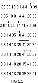
Consider the unsorted array,
a[1] a[2] a[8]
The resulting array should be
a[1] a[2] a[8]
One way to sort the unsorted array would be to perform the following steps:
- Find the smallest element in the unsorted array
- Place the smallest element in position of a[1]
i.e., the smallest element in the unsorted array is 3 so exchange the values of a[1] and a[7]. The array now becomes,
a[1] a[2] a[8]
Now find the smallest from a[2] to a[8] ,
i.e., 8 so exchange the values of a[2] and a[4] which results with the
array shown below,
a[1] a[2] a[8]
Repeat this process until the entire array is
sorted. The changes undergone by the array is shown in fig 2.2.The
number of moves with this technique is always of the order O(n).
 2.3.2 Insertion sort
Insertion
sort is a straight forward method that is useful for small collection
of data. The idea here is to obtain the complete solution by inserting
an element from the unordered part into the partially ordered solution
extending it by one element. Selecting an element from the unordered
list could be simple if the first element of that list is selected.
a[1] a[2] a[8]
Initially the whole array is unordered. So
select the minimum and put it in place of a[1] to act as sentinel. Now
the array is of the form,
a[1] a[2] a[8]
Now we have one element in the sorted list and
the remaining elements are in the unordered set. Select the next
element to be inserted. If the selected element is less than the
preceding element move the preceding element by one position and insert
the smaller element.
In the above array the next element to be
inserted is x=35, but the preceding element is 3 which is less than x.
Hence, take the next element for insertion i.e., 18. 18 is less than
35, so move 35 one position ahead and place 18 at that place. The
resulting array will be,
a[1] a[2] a[8]
Now the element to be inserted is 8. 8 is less
than 35 and 8 is also less than 18 so move 35 and 18 one position right
and place 8 at a[2]. This process is carried till the sorted array is
obtained.
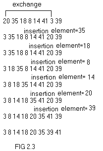 The changes undergone are shown in fig 2.3.
One of the disadvantages of the insertion sort
method is the amount of movement of data. In the worst case, the number
of moves is of the order O(n2). For lengthy records it is quite time consuming.
2.3.3 Merge sort The changes undergone are shown in fig 2.3.
One of the disadvantages of the insertion sort
method is the amount of movement of data. In the worst case, the number
of moves is of the order O(n2). For lengthy records it is quite time consuming.
2.3.3 Merge sort
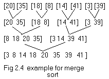 Merge sort begins by interpreting the inputs as n sorted files
each of length one. These are merged pair wise to obtain n/2 files of
size two. If n is odd one file is of size one. These n/2 files are then
merged pair wise and so on until we are left with only one file. The
example in fig 2.4 illustrates the process of merge sort.
As illustrated in the example merge sort
consists of several passes over the records being sorted. In the first
pass files of size one are merged. In the second pass the size of the
files being merged is two. In the ith pass the files being merged will be of size 2i-1. A total of log2n
passes are made over the data. Since, two files can be merged in linear
time, each pass of merge sort takes O(n) time. As there are log2n passes the total time complexity is O(n log2n). Merge sort begins by interpreting the inputs as n sorted files
each of length one. These are merged pair wise to obtain n/2 files of
size two. If n is odd one file is of size one. These n/2 files are then
merged pair wise and so on until we are left with only one file. The
example in fig 2.4 illustrates the process of merge sort.
As illustrated in the example merge sort
consists of several passes over the records being sorted. In the first
pass files of size one are merged. In the second pass the size of the
files being merged is two. In the ith pass the files being merged will be of size 2i-1. A total of log2n
passes are made over the data. Since, two files can be merged in linear
time, each pass of merge sort takes O(n) time. As there are log2n passes the total time complexity is O(n log2n). |
Recursion
|
|
|
Recursion may have the following definitions:
-The nested repetition of identical algorithm is recursion.
-It is a technique of defining an object/process by itself.
-Recursion is a process by which a function calls itself repeatedly until some specified condition has been satisfied.
2.4.1 When to use recursion
Recursion
can be used for repetitive computations in which each action is stated
in terms of previous result. There are two conditions that must be
satisfied by any recursive procedure.
- Each time a function calls itself it should get nearer to the solution.
- There must be a decision criterion for stopping the process.
In making the decision about whether to write
an algorithm in recursive or non-recursive form, it is always advisable
to consider a tree structure for the problem. If the structure is
simple then use non-recursive form. If the tree appears quite bushy,
with little duplication of tasks, then recursion is suitable.
The recursion algorithm for finding the factorial of a number is given below,
Algorithm : factorial-recursion
Input : n, the number whose factorial is to be found.
Output : f, the factorial of n
Method : if(n=0)
f=1
else
f=factorial(n-1) * n
if end
algorithm ends.
The general procedure for any recursive algorithm is as follows,
- Save the parameters, local variables and return addresses.
- If the termination criterion is reached
perform final computation and goto step 3 otherwise perform final
computations and goto step 1
 Restore the most recently saved parameters, local variable and return address and goto the latest return address. Restore the most recently saved parameters, local variable and return address and goto the latest return address.
2.4.2 Iteration v/s Recursion
Demerits of recursive algorithms
- Many programming languages do not
support recursion, hence recursive mathematical function is implemented
using iterative methods.
- Even though mathematical functions can
be easily implemented using recursion it is always at the cost of
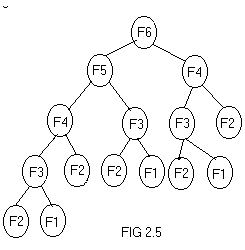
execution time and memory space. For example, the recursion tree for
generating 6 numbers in a fibonacci series generation is given in fig
2.5. A fibonacci series is of the form 0,1,1,2,3,5,8,13,
etc, where the
third number is the sum of preceding two numbers and so on. It can be
noticed from the fig 2.5 that, f(n-2) is computed twice, f(n-3) is
computed thrice, f(n-4) is computed 5 times.
- A recursive procedure can be called from
within or outside itself and to ensure its proper functioning it has to
save in some order the return addresses so that, a return to the proper
location will result when the return to a calling statement is made.
- The recursive programs needs considerably more storage and will take more time.
Demerits of iterative methods
- Mathematical functions such as factorial
and fibonacci series generation can be easily implemented using
recursion than iteration.
- In iterative techniques looping of statement is very much necessary.
Recursion is a top down approach to problem
solving. It divides the problem into pieces or selects out one key
step, postponing the rest.
Iteration is more of a bottom up approach. It
begins with what is known and from this constructs the solution step by
step. The iterative function obviously uses time that is O(n) where as
recursive function has an exponential time complexity.
It is always true that recursion can be
replaced by iteration and stacks. It is also true that stack can be
replaced by a recursive program with no stack.
2.5 Hashing
Hashing is a practical
technique of maintaining a symbol table. A symbol table is a data
structure which allows to easily determine whether an arbitrary element
is present or not.
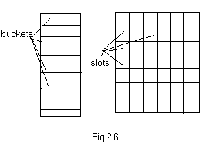
Consider a sequential memory shown in fig 2.6.
In hashing technique the address X of a variable x is obtained by
computing an arithmetic function (hashing function) f(x). Thus f(x)
points to the address where x should be placed in the table. This
address is known as the hash address.
The memory used to store the variable using
hashing technique is assumed to be sequential. The memory is known as
hash table. The hash table is partitioned into several storing spaces
called buckets and each bucket is divided into slots (fig 2.6).
If there are b buckets in the table, each
bucket is capable of holding s variables, where each variable occupies
one slot. The function f(x) maps the possible variable onto the
integers 0 through b-1. The size of the space from where the variables
are drawn is called the identifier space. Let T be the identifier
space, n be the number of variables/identifiers in the hash table.
Then, the ratio n/T is called the identifier density and a = n/sb is
the loading density or loading factor.

If f(x1)=f(x2), where x1and x2 are any two variables, then x1and x2 are
called synonyms. Synonyms are mapped onto the same bucket. If a new
identifier is hashed into a already complete bucket, collision occurs.
A hashing table with single slot is as given
below. Let there be 26 buckets with single slot. The identifier to be
stored are GA, D, A, G, L, A2, A1, A3, A4, Z, ZA, E. Let f(x) be the
function which maps on to a address equal to the position of the first
character of the identifier in the set of English alphabet. The hashing
table generated is as shown in fig 2.7.
Time taken to retrieve the identifiers is as follows,
|
Search element (x) |
Search time (t) |
|
GA |
1 |
|
D |
1 |
|
A |
1 |
|
G |
2 |
|
L |
1 |
|
A2 |
2 |
|
A1 |
3 |
|
A3 |
5 |
|
A4 |
6 |
|
Z |
1 |
|
ZA |
10 |
|
E |
6 |
| |
∑t =39 |
Average retrieval time =(∑t)/n.
The average retrieval time entirely depends on the hashing function.
Exercise 2:
- What are the serious short comings of the binary search method and sequential search method.
- Know more searching techniques involving hashing functions
- Implement the algorithms for searching and calculate the complexities
- Write an algorithm for the above method of selection sort and implement the same.
- Write the algorithm for merge sort method
- Take 5 data set of length 10 and hand simulate for each method given above.
- Try to know more sorting techniques and make a comparative study of them.
- Write an iterative algorithm to find the factorial of a number
- Write a recursive and iterative program for reversing a number
- Write recursive and iterative program to find maximum and minimum in a list of numbers.
- Write an algorithm to implement the hashing technique and implement the same
- Hand simulate all algorithms for a 5 datasets.
|
Post Resume: Click here to Upload your Resume & Apply for Jobs |

 Active Topics
  Memberlist
  Calendar
  Search
 Active Topics
  Memberlist
  Calendar
  Search
  Topic: Gate Study Material-Different perspectives of algo


 Topic: Gate Study Material-Different perspectives of algo
 IP Logged

