7.1 Single-source shortest path: Graphs can be used to represent the highway structure of a state or country with vertices representing cities and edges representing sections of highway. The edges can then be assigned weights which may be either the distance between the two cities connected by the edge or the average time to drive along that section of highway. A motorist wishing to drive from city A to B would be interested in answers to the following questions:

1. Is there a path from A to B?
2. If there is more than one path from A to B? Which is the shortest path?

The problems defined by these questions are special case of the path problem we study in this section. The length of a path is now defined to be the sum of the weights of the edges on that path. The starting vertex of the path is referred to as the source and the last vertex the destination. The graphs are digraphs representing streets. Consider a digraph G=(V,E), with the distance to be traveled as weights on the edges. The problem is to determine the shortest path from v0 to all the remaining vertices of G. It is assumed that all the weights associated with the edges are positive. The shortest path between v0 and some other node v is an ordering among a subset of the edges. Hence this problem fits the ordering paradigm.     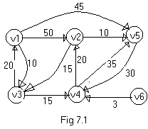Example: Consider the digraph of fig 7-1. Let the numbers on the edges be the costs of travelling along that route. If a person is interested travel from v1 to v2, then he encounters many paths. Some of them are

1. v1à v2 = 50 units
2. v1à v3à v4à v2 = 10+15+20=45 units
3. v1à v5à v4à v2 = 45+30+20= 95 units
4. v1à v3à v4à v5à v4à v2 = 10+15+35+30+20=110 units

The cheapest path among these is the path along v1à v3à v4à v2. The cost of the path is 10+15+20 = 45 units. Even though there are three edges on this path, it is cheaper than travelling along the path connecting v1 and v2 directly i.e., the path v1à v2 that costs 50 units. One can also notice that, it is not possible to travel to v6 from any other node. To formulate a greedy based algorithm to generate the cheapest paths, we must conceive a multistage solution to the problem and also of an optimization measure. One possibility is to build the shortest paths one by one. As an optimization measure we can use the sum of the lengths of all paths so far generated. For this measure to be minimized, each individual path must be of minimum length. If we have already constructed i shortest paths, then using this optimization measure, the next path to be constructed should be the next shortest minimum length path. The greedy way to generate these paths in non-decreasing order of path length. First, a shortest path to the nearest vertex is generated. Then a shortest path to the second nearest vertex is generated, and so on. A much simpler method would be to solve it using matrix representation. The steps that should be followed is as follows, Step 1: find the adjacency matrix for the given graph. The adjacency matrix for fig 7.1 is given below

	V1	V2	V3	V4	V5	V6
V1	-	50	10	Inf	45	Inf
V2	Inf	-	15	Inf	10	Inf
V3	20	Inf	-	15	inf	Inf
V4	Inf	20	Inf	-	35	Inf
V5	Inf	Inf	Inf	30	-	Inf
V6	Inf	Inf	Inf	3	Inf	-

Step 2: consider v1 to be the source and choose the minimum entry in the row v1. In the above table the minimum in row v1 is 10. Step 3: find out the column in which the minimum is present, for the above example it is column v3. Hence, this is the node that has to be next visited. Step 4: compute a matrix by eliminating v1 and v3 columns. Initially retain only row v1. The second row is computed by adding 10 to all values of row v3. The resulting matrix is

	V2	V4	V5	V6
V1à Vw	50	Inf	45	Inf
V1à V3à Vw	10+inf	10+15	10+inf	10+inf
Minimum	50	25	45	inf

Step 5: find the minimum in each column. Now select the minimum from the resulting row. In the above example the minimum is 25. Repeat step 3 followed by step 4 till all vertices are covered or single column is left. The solution for the fig 7.1 can be continued as follows

	V2	V5	V6
V1à Vw	50	45	Inf
V1à V3à V4à Vw	25+20	25+35	25+inf
Minimum	45	45	inf

 

	V5	V6
V1à Vw	45	Inf
V1à V3à V4à V2à Vw	45+10	45+inf
Minimum	45	inf

	V6
V1à Vw	Inf
V1à V3à V4à V2à V5à Vw	45+inf
Minimum	inf

Finally the cheapest path from v1 to all other vertices is given by V1à V3à V4à V2à V5.

click here for more details:
http://www.vyomworld.com/gate/cs/ada/7.1.asp